First Simulation
This tutorial walks through one simulation from an empty window to a
plotted waveform. It uses tran-simple-01.cir, a small series RLC circuit
that ships in the repository's netlists/
directory:
V1 IN 0 PULSE(0 5 0 1n 1n 10m 20m)
R1 IN N1 100
L1 N1 N2 10mH
C1 N2 0 1uF

.PREPROCESS REPLACEGROUND TRUE
.TRAN 1u 20m 0
.PRINT TRAN FORMAT=RAW FILE=tran-simple-01.raw V(*) I(*) P(*)
.FFT I(L1) NP=1024 WINDOW=HANN
.FFT I(C1) NP=1024 WINDOW=HANN
.FFT I(C1) NP=2048 WINDOW=HANN FORMAT=UNORM

.END
It is a 5 V pulse source driving a series R-L-C ladder, simulated for 20 ms of transient response.
Before you start
- Xyce is installed on your machine (see Installation).
- Xyce Studio runs and its executable path is configured (see Configuring the Xyce Executable).
1. Open the netlist
Launch Xyce Studio in standalone mode. Click Open in the toolbar and
select tran-simple-01.cir (or any other netlist file you have).
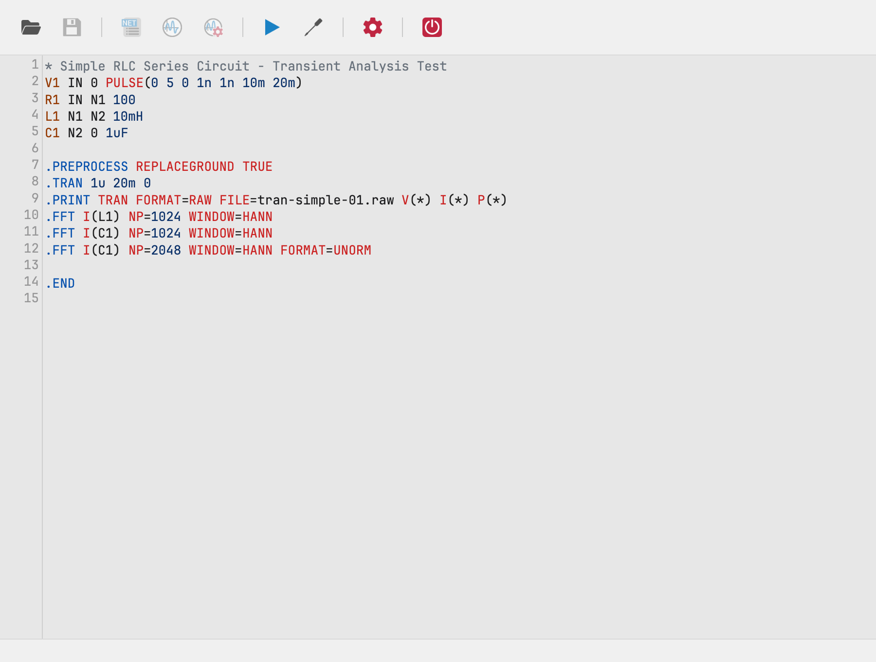
The netlist appears in the editor with line numbers and coloring. You can
change values before running: for example, change 10mH to 5mH — the
window title shows a * prefix when there are unsaved edits, and the
Save tool persists them to the .cir file.
2. Configure the analysis
The netlist already contains its own .TRAN line, so you could run it
as-is. To configure the analysis from the UI instead, click
Configure:
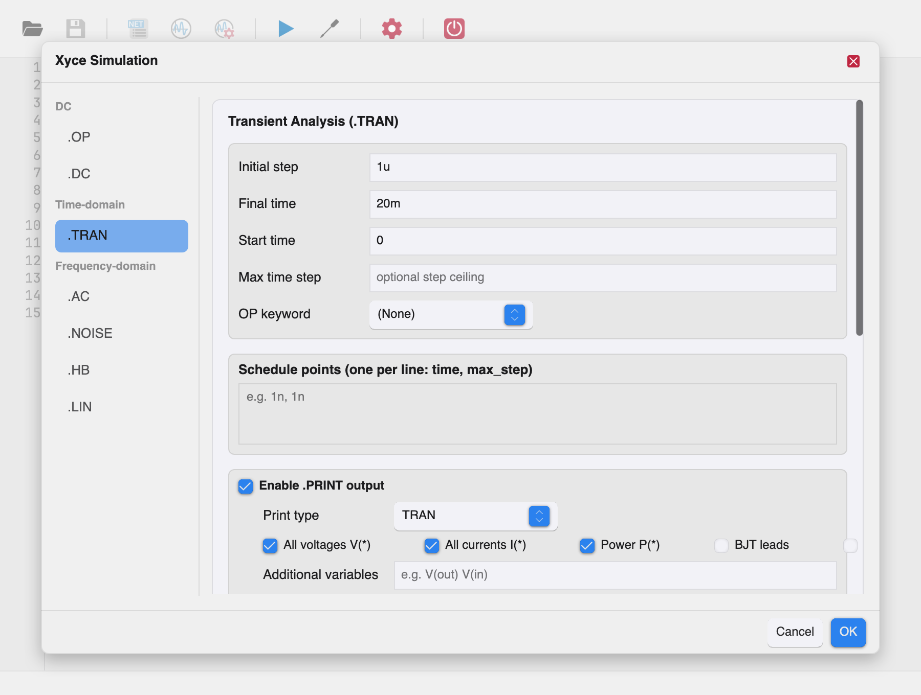
Set Initial step to 1u and Final time to 20m, enable
.PRINT output, and click OK. The resulting directives are merged
into the netlist before .END, and the simulation runs with them.
3. Run the simulation
Click Run Simulation. While the run is in flight the status bar shows
a progress bar with the completion percentage, the estimated time to
completion, and the warnings and errors Xyce has reported so far; click
the status bar to open the simulation output panel and watch the live
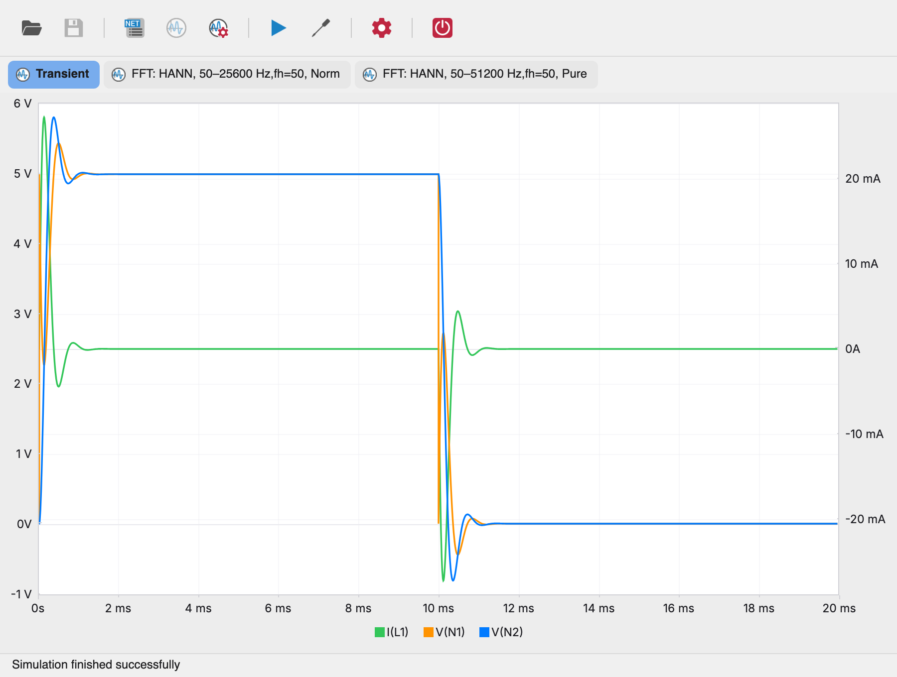
log. When the run ends the status bar reports Simulation finished
successfully and the charts panel opens automatically.
4. Plot some signals
A fresh chart starts empty: right-click the chart and choose
Add/Remove Plots to pick what to display. The expressions available
come from the .PRINT line — this run prints all node voltages and
device currents.
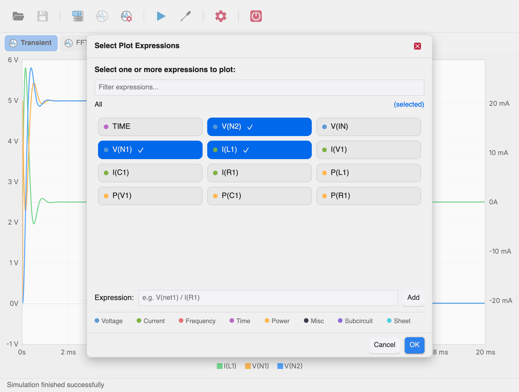
Click a couple of expression chips (for example V(IN) and V(N2)),
then OK. Each signal becomes a colored series with a legend below the
chart.
To skip this step on every run, add a
.PLOT line to the netlist, e.g.
.PLOT V(IN) V(N2), and the run opens with that chart already plotted.
5. Inspect the waveform
Hover the plot to read values in the status bar, and drag a rectangle inside the chart to zoom into a region — other charts in the tab follow the same horizontal window, which makes comparing signals easy.
6. Modify and rerun
Edit the netlist (for example change the pulse period from 20m to
40m), click Save, then Run Simulation again. New results
replace the previous ones and the charts refresh.
If something goes wrong — Xyce reports a parse error, or the charts stay empty — check the Troubleshooting page and the output shown by the Sim Output toolbar tool.